Data

Data is the lifeblood of any quantitative or systematic strategy. Before you can do any testing, you need to get data into the system. But first, there are a few foundational classes you will need to understand.

TimeSeries

A TimeSeries encapsulates an array of numeric values as well as their associated dates. In fact, TimeSeries act just like arrays in other programming languages so you can reference values via an indexer like [0]. Typically you won’t create a TimeSeries directly but rather will load data from a file or call an indicator that returns a TimeSeries object. For example, loading a csv file with a date and observation on each line is as simple as calling:

var ts = TimeSeries.Load(@"c:\data\MOVE Index.csv");

You can then examine several properties of interest:

ts.Count //number of observations
ts.FirstDate //first date in the series
ts.LastDate //last date in the series
ts.Symbol //symbol inferred from the filename

As well as visualize the data by calling the Chart() extension method:

ts.Chart();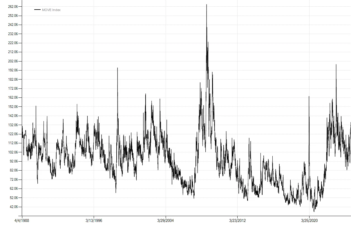

Bars and BarSeries

The next foundational class is the Bar. The standard Bar class contains Date, Open, High, Low, Close, Volume, OpenInterest, and UnadjustedClose properties. ContinuousBar is used for continuous futures data and extends the Bar class by adding a DeliveryDate property. The Bar class is extensible by design so additional fields can be included beyond the defaults. For example, you could load the S&P 500 OHLC (open, high, low, close) and also include the dividend yield as an extended property.

Like TimeSeries, we typically won’t create bars directly, but rather will load them from a data source. A single bar in isolation is of little use, so we will be working with BarSeries, a collection of bars ordered by date. Along with TimeSeries, BarSeries are one of the most commonly used data classes. Backtests run on BarSeries. Just like TimeSeries, you can load BarSeries directly from a text file:

var data = BarSeries.Load(@"c:\data\BCOM Index.csv");

//you can enumerate bars
foreach (var bar in data.Take(10))
{
    Console.WriteLine(bar);
}

//or get a TimeSeries of just the bar's closing prices
var close = data.Close;
//and of course you can chart a BarSeries as well
data.Chart();

Other series

• BooleanSeries contain true/false values and are commonly used to indicate a distinct event, for example when an indicator value crosses above a certain level.

• IntegerSeries work just like TimeSeries but store integer values instead of floating point double values.

• DateSeries encapsulate a list of dates only. This can be useful in backtesting for keeping track of dates that correspond to events like FOMC announcements or economic releases.

Futures Data

Futures contracts have a finite life. Therefore, system testing is often done using continuous or “backadjusted” contracts. Backadjusting is a process by which individual futures contracts are spliced together to create one continuous series. This continuous series replicates the P&L of holding a futures contract while rolling it from month-to-month. Below is an example of what historical futures data might look like:

Date	Open	High	Low	Close	Volume	Open Interest	Unadjusted Close	Delivery
19840913	663.07	666.70	661.85	666.55	73100	33100	169.30	Sep-84
19840914	667.35	668.25	665.95	666.40	73800	33600	169.15	Sep-84
19840917	666.60	667.35	665.60	666.55	64300	37000	173.00	Dec-84
19840918	666.35	667.05	665.55	666.15	63700	37900	172.60	Dec-84

On 9/17/1984 there was a roll from the September contract to the December contract. Note the unadjusted close on September 17th at 173 versus 666.55 for the backadjusted close. The unadjusted close is the price that existed at that point in time, free of the cumulative effects of backadjusting. Having the unadjusted close is critical for calculating accurate percentage changes, especially as the amount of history increases.

One common mistake is calculating percentage changes directly on backadjusted prices. The correct calculation for the percent change on 9/17/1984 is the point change in the backadjusted closing prices divided by the unadjusted close from the prior day:

• (666.55 - 666.40) / 169.15 = 0.000887

not

• 666.55 / 666.40 - 1 = 0.000225

and also not the change in unadjusted closes because of the roll on that date

• 173.00 / 169.15 - 1 = 0.022760

Considering that backadjusted prices can actually go negative, which introduces even more severe distortions to percentage calculations, it is important to be aware of this. Fortunately the backtester automatically uses the unadjusted close as the denominator whenever appropriate and when available in the data source.