Missing the Top
“Missing the bottom on the way up won’t cost you anything. It’s missing the top on the way down that’s always expensive.” Peter Lynch
I came across this quote recently in a The Saltwater Highway: One Man’s Journey through the International Dry Bulk Maritime Marke on maritime shipping. Peter Lynch’s “One Up on Wall Street” happened to be the first investment book I ever read. This quote has stuck with me the past few days as the S&P has sold off materially for the first time in months. In the age of FOMO, where risk is defined as missing out on the upside, this advice seemed surprising. Today, long-only fund managers are almost always fully invested. Lynch’s successor to the Magellan Fund, Jeffrey Vinik, ultimately left Fidelity after turning prematurely bearish in the mid-90’s, a lesson that other fund managers took to heart.
The second investment book I ever read was Martin Zweig’s “Winning On Wall Street”. This proved to be much more up my alley. Zweig described many quantitative methods including several trend-following systems, one of which was his 4% rule which he credited to Ned Davis. Prior to Davis, Arthur Merrill had done similar work with his “filtered waves”. The basic idea is to buy when the market rallies x% off a low and sell when it falls y% from a high. The buy and sell thresholds can be symmetrical, as in the Zweig 4% rule, or they can vary.
Recently I had been doing work on past major bear markets using some long-term total return data (more technical work for a future blog post perhaps). This seemed like the perfect dataset on which to test the filter rule and quantify Lynch’s contention. The data starts in 1973 and ends in late 2021. Countries include Australia, Canada, Germany, Europe ex UK, Hong Kong, Japan, United Kingdom, and the United States.
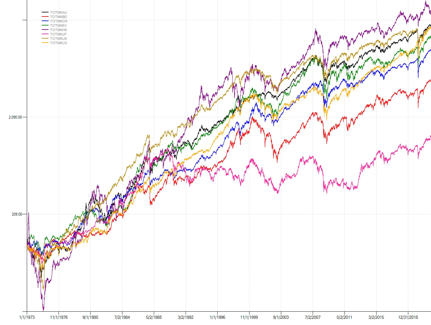 Data source: Datastream
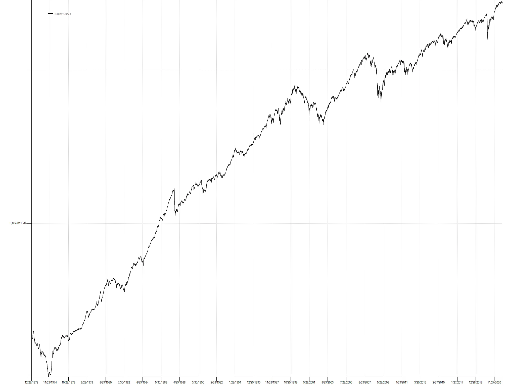
Before we can test the filter rule, we need a benchmark with which to compare results. I took the eight total return streams, assumed they were all priced in USD for simplicity, equally weighted them at a 12.5% portfolio weight, and rebalanced to target once a year to arrive at a buy and hold benchmark. It delivers a 10.5% compound annual return but with a fairly punishing -53.5% drawdown. Despite what recent history might suggest, large drawdowns are par for the course for equities over the long run. The portfolio Sharpe of 0.91 is a material improvement over the best stand-alone market Sharpe of 0.66 thanks to diversification (and to a lesser degree the annual rebalancing).
| Strategy: | Buy & Hold |
|---|---|
| CAGR | 10.55% |
| Volatility | 11.63% |
| Max Drawdown | -53.49% |
| Sharpe Ratio | 0.91 |
| MAR Ratio | 0.20 |
| Ulcer Performance Index | 0.72 |
Equally weighted buy & hold portfolio equity curve:
Next using the same eight markets, I applied the filter logic. Using Zweig’s 4% rule as an example, we would buy the first time a market’s total return index rallied 4% from a closing low. We hold that long position until it falls 4% from the highest close observed over the life of the trade at which point we sell. I tested buy and sell percentage thresholds independently from 3% to 20% in 1% increments.
These backtests have a heroic number of simplifying assumptions:
- I assume an arbitrary 20 bps in transaction costs as a speedbump to penalize frequent trading.
- I again ignore FX conversions and assume each total return index is priced in USD.
- All trades are executed on the close of the signal bar.
- When the filter logic signals an exit we move to cash. No interest is accrued.
- Positions are sized at 12.5% of equity at the time of entry without any additional rebalancing.
The goal is to analyze the general efficacy of the filter logic, not to provide the most accurate backtest possible (which is exceedingly difficult over very long timeframes). The table below shows the top ten buy/sell threshold parameters sorted by Sharpe Ratio out of the 324 parameter combinations tested.
| Buy Threshold | Sell Threshold | CAGR | Volatility | Sharpe Ratio | MAR Ratio | Ulcer Performance Index | Max Drawdown % | Trades | % Profitable |
|---|---|---|---|---|---|---|---|---|---|
| 12% | 8% | 9.59% | 7.09% | 1.35 | 0.30 | 1.25 | -31.73% | 453 | 51.4% |
| 11% | 8% | 9.86% | 7.33% | 1.35 | 0.33 | 1.27 | -29.67% | 485 | 50.5% |
| 10% | 8% | 10.15% | 7.56% | 1.34 | 0.32 | 1.23 | -31.30% | 518 | 50.6% |
| 13% | 8% | 9.27% | 6.91% | 1.34 | 0.32 | 1.32 | -28.95% | 431 | 52.4% |
| 14% | 8% | 8.96% | 6.73% | 1.33 | 0.38 | 1.44 | -23.60% | 407 | 54.5% |
| 13% | 9% | 9.64% | 7.29% | 1.32 | 0.32 | 1.25 | -30.20% | 392 | 53.1% |
| 12% | 9% | 9.86% | 7.48% | 1.32 | 0.29 | 1.16 | -33.94% | 413 | 51.8% |
| 11% | 9% | 10.13% | 7.70% | 1.32 | 0.31 | 1.20 | -32.52% | 438 | 49.8% |
| 10% | 9% | 10.39% | 7.92% | 1.31 | 0.30 | 1.17 | -34.62% | 465 | 50.5% |
| 19% | 8% | 7.62% | 5.83% | 1.31 | 0.36 | 1.34 | -21.19% | 318 | 57.5% |
The optimal Sharpe of 1.35 represents a 48% improvement over the benchmark. Maximum drawdown is significantly reduced from over -50% to approximately -30%, which makes it much easier to recover to new equity highs (remember the punishing logic of percentages whereby a 50% decline requires a 100% gain to get back to even). But most interesting to me are the buy and sell thresholds that bubble to the top. The optimal strategy is to be relatively slow to buy but quicker to sell, just as Peter Lynch advises. And note you don’t have to be on a hair trigger either: an 8% to 9% sell threshold is optimal. To put that into context, this week’s sell off in the cash S&P, which has already generated a lot of angst and headlines, only brought the index down 4.24% off its closing high, roughly half-way to the optimal sell threshold.
This is certainly contrary to how most people operate where they are quick to buy and slow to sell (if at all). Most professional fund managers would never contemplate a strategy like this. They simply can’t. The FOMO and client pressure won’t let them. Imagine sitting on the sidelines while the market rallies 10 to 15%. You finally get in only to have the market reverse down 8%. But if you want to outperform, you have to do something different. Nobody ever promised it would be easy which is why having a systematic approach (and a very long time horizon) can help.
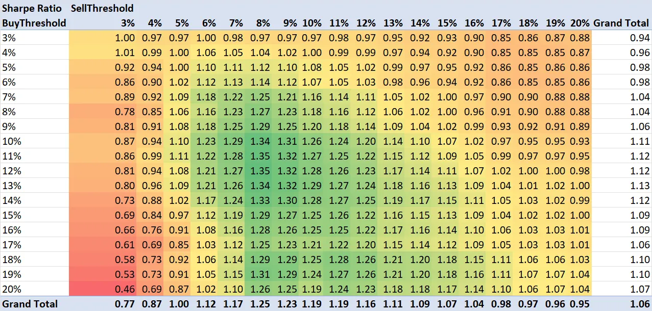
The other interesting thing about the filter system is it is relatively stable across a reasonable parameter range. The pivot table below shows the Sharpe Ratio for each buy/sell threshold combination. 83% of parameter combinations outperform the buy and hold benchmark. The average Sharpe across the full parameter space is 1.06, also better than the benchmark.
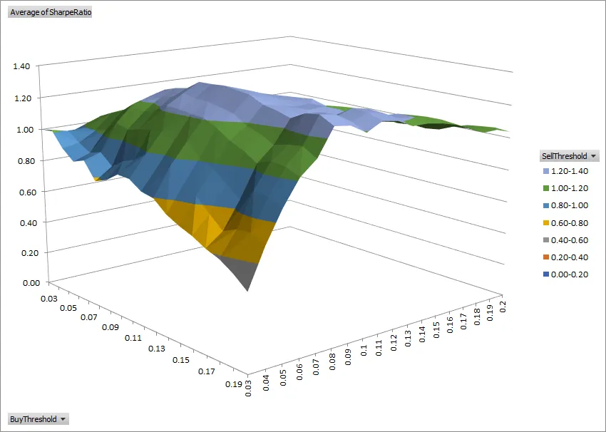
The surface chart plots the Sharpe Ratio with respect to the buy threshold (left-hand axis) and the sell threshold (right-hand axis). Here we can visualize the plateau of stable performance as well as the degradation that occurs as the sell threshold approaches 3%, a level below which noise starts to dominate.
The list of caveats to implementing this system would be as lengthy as this blog post, not the least of which are taxes, which are rarely discussed. But interesting nonetheless to see an investing legend’s qualitative advice reflected in the numbers and yet so contrary to the received wisdom of the day. If you are feeling pressure that you missed the top in the S&P, you may have, but if you are applying trend following to equities with an eye over the very long term, the jury is still out.
class FilterRule : Strategy{    public static void Run()    {        AsciiBarServer server = new AsciiBarServer(@"c:\data\globalIndices", AsciiBarServer.DC);        var data = server.LoadAll(new DateTime(1973, 1, 1));
        var strat = new BuyAndHold();        strat.MoneyManager = new AnnualRebalance();        strat.RunSimulation(data);
        var vd = new VariableDictionary();        vd["TransactionCosts"] = new BasisPointTransactionCosts { BasisPoints = 20 };
        var opt = new Optimizer() { AutoExport = false };        opt.Optimize(typeof(FilterRule), vd, typeof(EquallyWeighted), null, data);        opt.GetResults().Rank().ExportToExcel();    }
    [Optimize(0.03, 0.2, 0.01)]    public double BuyThreshold { get; set; } = 0.04;
    [Optimize(0.03, 0.2, 0.01)]    public double SellThreshold { get; set; } = 0.04;
    protected override void OnStrategyStart()    {        Col1 = Indicators.Filter(Close, BuyThreshold, SellThreshold, true);    }
    protected override void OnBarClose()    {        if (Col1.Last == 1)        {            BuyClose();        }        else        {            SellClose();        }    }}
class AnnualRebalance : EquallyWeighted{    protected override void OnMarketClosing()    {        base.OnMarketClosing();
        if (DateHelper.IsYearEnd(CurrentDate))        {            foreach (var position in OpenPositions)            {                var target = (Equity + ChangeToday) / NumberOfPositions / position.Last;                Rebalance(position, target)            }        }    }}